Regression and inference

# Regression and inference

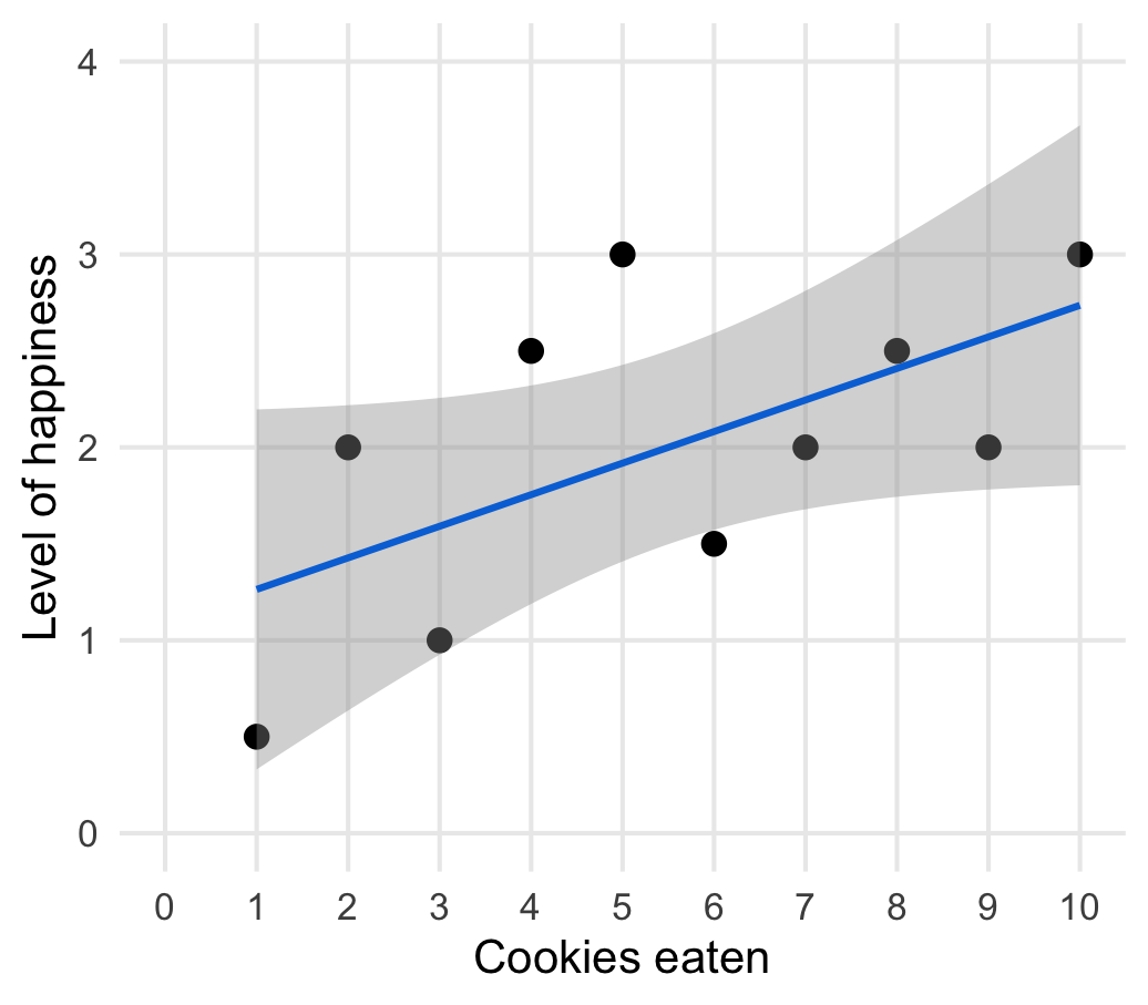
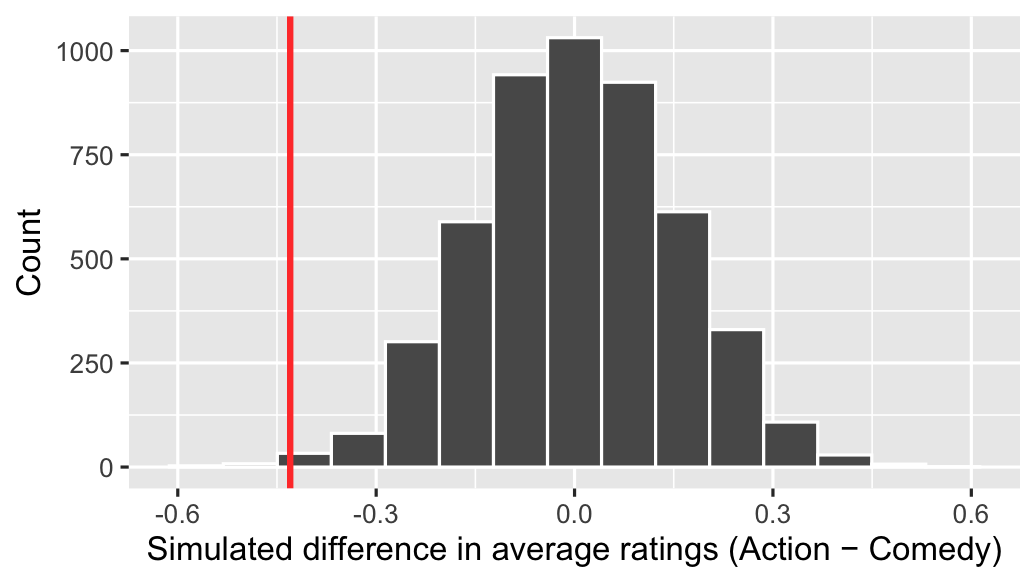
**Session 2**

]

---

# Plan for today

.box-2.medium.sp-after-half[Drawing lines]

.box-6.medium.sp-after-half[Lines, Grϵϵκ, and regression]

.box-5.medium.sp-after-half[Null worlds and statistical significance]

---

layout: false
name: drawing-lines
class: center middle section-title section-title-2 animated fadeIn

# Drawing lines

---

---

# Essential parts of regression

---

# Identify variables

.box-inv-2[Researchers predict genocides by looking at negative media coverage, revolutions in neighboring countries, and economic growth]
]

.pull-right[
.box-inv-2[You want to see if taking more AP classes in high school improves college grades]

.box-inv-2[Netflix uses your past viewing history, the day of the week, and the time of the day to guess which show you want to watch next]
]

---

# Two purposes of regression

.box-2.sp-after[Focus is on **Y**]

.box-inv-2.small[Netflix trying to guess your next show]

.box-inv-2.small[Predicting who will enroll in SNAP]
]

.box-2.sp-after[Focus is on **X**]

.box-inv-2.small[Netflix looking at the effect of the time of day on show selection]

.box-inv-2.small[Measuring the effect of SNAP on poverty reduction]
]

---

# How?

.box-inv-2.medium.sp-after-half[Plot **X** and **Y**]

.box-inv-2.medium[Draw a line that approximates the relationship]

.box-2.tiny[and that would plausibly work for data not in the sample!]

.box-inv-2.medium.sp-after-half.sp-before-half[Find mathy parts of the line]

.box-inv-2.medium[Interpret the math]

---

# Cookies and happiness

```
## # A tibble: 10 × 2
## happiness cookies
## <dbl> <int>
## 1 0.5 1
## 2 2 2
## 3 1 3
## 4 2.5 4
## 5 3 5
## 6 1.5 6
## 7 2 7
## 8 2.5 8
## 9 2 9
## 10 3 10
```

]

---

---

---

---

---

---

---

---

# Ordinary least squares (OLS) regression

---

layout: false
name: lines-greek-regression
class: center middle section-title section-title-6 animated fadeIn

# Lines, Grϵϵκ, and regression

---

---

# Drawing lines with math

$$
y = mx + b
$$

<table>
 <tr>
 <td class="cell-center">$y$</td>
 <td class="cell-left">&ensp;A number</td>
 </tr>
 <tr>
 <td class="cell-center">$x$</td>
 <td class="cell-left">&ensp;A number</td>
 </tr>
 <tr>
 <td class="cell-center">$m$</td>
 <td class="cell-left">&ensp;Slope ($\frac{\text{rise}}{\text{run}}$)</td>
 </tr>
 <tr>
 <td class="cell-center">$b$</td>
 <td class="cell-left">&ensp;y-intercept</td>
 </tr>
</table>

---

# Slopes and intercepts

$$
y = 2x - 1
$$

]

$$
y = -0.5x + 6
$$

]

---

# Greek, Latin, and extra markings

Letters like `$\beta_1$` are the ***truth***

Letters with extra markings like `$\hat{\beta_1}$` are our ***estimate*** of the truth based on our sample
]

Letters like `$X$` are ***actual data*** from our sample

Letters with extra markings like `$\bar{X}$` are ***calculations*** from our sample
]

---

# Estimating truth

.box-inv-6.sp-after[Data → Calculation → Estimate → Truth]

.pull-left[
<table>
 <tr>
 <td class="cell-left">Data</td>
 <td class="cell-center">$X$</td>
 </tr>
 <tr>
 <td class="cell-left">Calculation&ensp;</td>
 <td class="cell-center">$\bar{X} = \frac{\sum{X}}{N}$</td>
 </tr>
 <tr>
 <td class="cell-left">Estimate</td>
 <td class="cell-center">$\hat{\mu}$</td>
 </tr>
 <tr>
 <td class="cell-left">Truth</td>
 <td class="cell-center">$\mu$</td>
 </tr>
</table>
]

$$
X \rightarrow \bar{X} \rightarrow \hat{\mu} \xrightarrow{\text{🤞 hopefully 🤞}} \mu
$$
]

---

# Drawing lines with stats

$$
\hat{y} = \hat{\beta_0} + \hat{\beta_1} x_1 + \varepsilon
$$

<table>
 <tr>
 <td class="cell-center">$y$</td>
 <td class="cell-center">$\hat{y}$</td>
 <td class="cell-left">&ensp;Outcome variable (DV)</td>
 </tr>
 <tr>
 <td class="cell-center">$x$</td>
 <td class="cell-center">$x_1$</td>
 <td class="cell-left">&ensp;Explanatory variable (IV)</td>
 </tr>
 <tr>
 <td class="cell-center">$m$</td>
 <td class="cell-center">$\hat{\beta_1}$</td>
 <td class="cell-left">&ensp;Slope</td>
 </tr>
 <tr>
 <td class="cell-center">$b$</td>
 <td class="cell-center">$\hat{\beta_0}$</td>
 <td class="cell-left">&ensp;y-intercept</td>
 </tr>
 <tr>
 <td class="cell-center">&emsp;&emsp;</td>
 <td class="cell-center">&emsp;$\varepsilon$&emsp;</td>
 <td class="cell-left">&ensp;Error (residuals)</td>
 </tr>
</table>

.box-inv-6.smaller[(most of the time we can get rid of markings on Greek and just use β)]

---

# Modeling cookies and happiness

$$
`\begin{aligned}
&\widehat{\text{happiness}} = \\ 
&\beta_0 + \beta_1 \text{cookies} + \varepsilon
\end{aligned}`
$$

]

]

---

# Building models in R

```r
name_of_model <- lm(<Y> ~ <X>, data = <DATA>)

summary(name_of_model)  # See model details
```

```r
library(broom)

# Convert model results to a data frame for plotting
tidy(name_of_model)

# Convert model diagnostics to a data frame
glance(name_of_model)
```

---

# Modeling cookies and happiness

.pull-left[
$$
`\begin{aligned}
&\widehat{\text{happiness}} = \\ 
&\beta_0 + \beta_1 \text{cookies} + \varepsilon
\end{aligned}`
$$

```r
happiness_model <- 
 lm(happiness ~ cookies,
 data = cookies_data)
```

]

---

# Modeling cookies and happiness

```r
tidy(happiness_model, conf.int = TRUE)
```

```
## # A tibble: 2 × 7
## term estimate std.error statistic p.value conf.low conf.high
## <chr> <dbl> <dbl> <dbl> <dbl> <dbl> <dbl>
## 1 (Intercept) 1.1 0.470 2.34 0.0475 0.0156 2.18 
## 2 cookies 0.164 0.0758 2.16 0.0629 -0.0111 0.338
```
]

```r
glance(happiness_model)
```

```
## # A tibble: 1 × 12
## r.squ…¹ adj.r…² sigma stati…³ p.value df logLik AIC BIC devia…⁴ df.re…⁵
## <dbl> <dbl> <dbl> <dbl> <dbl> <dbl> <dbl> <dbl> <dbl> <dbl> <int>
## 1 0.368 0.289 0.688 4.66 0.0629 1 -9.34 24.7 25.6 3.79 8
## # … with 1 more variable: nobs <int>, and abbreviated variable names
## # ¹r.squared, ²adj.r.squared, ³statistic, ⁴deviance, ⁵df.residual
## # ℹ Use `colnames()` to see all variable names
```
]

---

# Translating results to math

```
## # A tibble: 2 × 2
## term estimate
## <chr> <dbl>
## 1 (Intercept) 1.1 
## 2 cookies 0.164
```
]

.small[
$$
`\begin{aligned}
&\widehat{\text{happiness}} = \\ 
&\beta_0 + \beta_1 \text{cookies} + \varepsilon
\end{aligned}`
$$

$$
`\begin{aligned}
&\widehat{\text{happiness}} = \\ 
&1.1 + 0.16 \times \text{cookies} + \varepsilon
\end{aligned}`
$$
]
]

---

# Template for single variables

.box-inv-6.medium[A one unit increase in X is *associated* with a β1 increase (or decrease) in Y, on average]

$$
\widehat{\text{happiness}} = \beta_0 + \beta_1 \text{cookies} + \varepsilon
$$

$$
\widehat{\text{happiness}} = 1.1 + 0.16 \times \text{cookies} + \varepsilon
$$

---

# Multiple regression

$$
\hat{y} = \beta_0 + \beta_1 x_1 + \beta_2 x_2 + \cdots + \beta_n x_n + \varepsilon
$$

&nbsp;

```r
car_model <- lm(hwy ~ displ + cyl + drv,
 data = mpg)
```

$$
\widehat{\text{hwy}} = \beta_0 + \beta_1 \text{displ} + \beta_2 \text{cyl} + \beta_3 \text{drv:f} + \beta_4 \text{drv:r} + \varepsilon
$$

---

# Modeling lots of things and MPG

```r
tidy(car_model, conf.int = TRUE)
```

```
## # A tibble: 5 × 7
## term estimate std.error statistic p.value conf.low conf.high
## <chr> <dbl> <dbl> <dbl> <dbl> <dbl> <dbl>
## 1 (Intercept) 33.1 1.03 32.1 9.49e-87 31.1 35.1 
## 2 displ -1.12 0.461 -2.44 1.56e- 2 -2.03 -0.215
## 3 cyl -1.45 0.333 -4.36 1.99e- 5 -2.11 -0.796
## 4 drvf 5.04 0.513 9.83 3.07e-19 4.03 6.06 
## 5 drvr 4.89 0.712 6.86 6.20e-11 3.48 6.29
```
]

$$
`\begin{aligned}
\widehat{\text{hwy}} =&\ 33.1 + (-1.12) \times \text{displ} + (-1.45) \times \text{cyl} \ + \\
&(5.04) \times \text{drv:f} + (4.89) \times \text{drv:r} + \varepsilon
\end{aligned}`
$$

---

# Sliders and switches

.center[
<figure>
 <img src="img/02/slider-switch-plain-80.jpg" alt="Switch and slider" title="Switch and slider" width="100%">
</figure>
]

---

# Sliders and switches

.center[
<figure>
 <img src="img/02/slider-switch-annotated-80.jpg" alt="Switch and slider" title="Switch and slider" width="100%">
</figure>
]

---

# Filtering out variation

.box-inv-6.medium.sp-after[Each **X** in the model explains some portion of the variation in **Y**]

.box-6[Interpretation is a little trickier, since you can only ever move **one** switch or slider at at time]

---

# Template for continuous variables

.box-inv-6[*Holding everything else constant*, a one unit increase in **X** is *associated* with a βn increase (or decrease) in **Y**, on average]

.box-6.small[On average, a one unit increase in cylinders is associated with 1.45 lower highway MPG, holding everything else constant]

---

# Template for categorical variables

.box-inv-6[*Holding everything else constant*, **Y** is βn units larger (or smaller) in **X**n, compared to **X**omitted, on average]

.box-6[On average, front-wheel drive cars have 5.04 higher highway MPG than 4-wheel-drive cars, holding everything else constant]

---

# Economists and Greek letters

$$
Y_i = \alpha + \beta P_i + \gamma A_i + e_i
$$

.box-inv-6.tiny[Equation 2.1 on p. 57 in *Mastering 'Metrics*]

.box-6.smaller[*i* = an individual]

.box-6.smaller[α ("alpha") = intercept]

.box-6.smaller[β ("beta") = coefficient just for *treatment*, or the causal effect]

.box-6.smaller[γ ("gamma") = coefficient for the *identifying variable* (being in Group A or not)]

---

# Economists and Greek letters

$$
\ln Y_i = \alpha + \beta P_i + \gamma A_i + \delta_1 \text{SAT}_i + \delta_2 \text{PI}_i + e_i
$$

.box-inv-6.tiny[Equation 2.2 on p. 61 in *Mastering 'Metrics*]

.box-6.small[*i* = an individual]

.box-6.small[α ("alpha") = intercept]

.box-6.small[β ("beta") = coefficient just for *treatment*, or the causal effect]

.box-6.small[γ ("gamma") = coefficient for the *identifying variable* (being in Group A or not)]

.box-6.small[δ ("delta") = coefficient for *control variables*]

---

# These are all the same thing!

$$
\ln Y_i = \alpha + \beta P_i + \gamma A_i + \delta_1 \text{SAT}_i + \delta_2 \text{PI}_i + e_i
$$

$$
\ln Y_i = \beta_0 + \beta_1 P_i + \beta_2 A_i + \beta_3 \text{SAT}_i + \beta_4 \text{PI}_i + e_i
$$

```r
lm(log(income) ~ private + group_a + sat + parental_income, 
   data = income_data)
```

.box-inv-6[(I personally like the all-β version instead of using like the entire Greek alphabet, but you'll see both varieties in the real world)]

---

layout: false
name: significance
class: center middle section-title section-title-5 animated fadeIn

# Null worlds and statistical significance

---

---

# "hopefully"

.box-inv-5.medium[How do we know if our estimate is the truth?]

$$
X \rightarrow \bar{X} \rightarrow \hat{\mu} \xrightarrow{\text{🤞 hopefully 🤞}} \mu
$$

---

.box-inv-5.medium.sp-after[Are action movies rated higher than comedies?]

<table>
 <tr>
 <td class="cell-left">Data</td>
 <td class="cell-left">IMDB ratings</td>
 <td class="cell-center">$D$</td>
 </tr>
 <tr>
 <td class="cell-left">Calculation&ensp;</td>
 <td class="cell-left">Average action rating − average comedy rating</td>
 <td class="cell-center">$\bar{D} = \frac{\sum{D}_\text{Action}}{N} - \frac{\sum{D}_\text{Comedy}}{N}$</td>
 </tr>
 <tr>
 <td class="cell-left">Estimate</td>
 <td class="cell-left">$\bar{D}$ in a sample of movies</td>
 <td class="cell-center">$\hat{\delta}$</td>
 </tr>
 <tr>
 <td class="cell-left">Truth</td>
 <td class="cell-left">Difference in rating for all movies</td>
 <td class="cell-center">$\delta$</td>
 </tr>
</table>

---

```r
head(movie_data)
```

```
## # A tibble: 6 × 4
## title year rating genre 
## <chr> <int> <dbl> <fct> 
## 1 Tarzan Finds a Son! 1939 6.4 Action
## 2 Silmido 2003 7.1 Action
## 3 Stagecoach 1939 8 Action
## 4 Diamondbacks 1998 1.9 Action
## 5 Chaos Factor, The 2000 4.5 Action
## 6 Secret Command 1944 7 Action
```
]

```r
movie_data %>% 
  group_by(genre) %>% 
  summarize(avg_rating = mean(rating))
```

```
## # A tibble: 2 × 2
## genre avg_rating
## <fct> <dbl>
## 1 Action 5.41
## 2 Comedy 5.84
```

$$
\hat{\delta} = \bar{D} = 5.41 - 5.84 = 0.43
$$
.box-5[Is the true δ 0.43?]
]

---

---

# Null worlds

.box-inv-5.medium[What would the world look like if the true δ was really 0?]

.box-5[Action movies and comedies wouldn't all have the same rating, but on average there'd be no difference]

---

# Simulated null world

.box-inv-5[Shuffle the `rating` and `genre` columns and calculate the difference in ratings across genres]

.center[
<img src="02-slides_files/figure-html/plot-null-1.png" width="50%" style="display: block; margin: auto;" />
]

---

# Check δ in the null world

.center[
<img src="02-slides_files/figure-html/plot-null-delta-1.png" width="50%" style="display: block; margin: auto;" />
]

---

# How likely is that δ in the null world?

.pull-right[
.box-inv-5[What's the chance that we'd see that red line in a world where there's no difference?]

---

# p-values

.box-inv-5.sp-after[p-value = probability of seeing something in a world where the effect is 0]

.box-5[We can safely say that there's a difference between the two groups. Action movies are rated lower, on average, than comedies]

---

# Significance

.box-inv-5.sp-after[If p < 0.05, there's a good chance the estimate is not zero and is "real"]

---

# No need for all that simulation

.box-inv-5.small[This simulation stuff is helpful for the intuition behind a p-value, but you can also just interpret p-values in the wild]

```r
t.test(rating ~ genre, data = movie_data)
```

```
## 
## 	Welch Two Sample t-test
## 
## data:  rating by genre
## t = -2.8992, df = 388.75, p-value = 0.003953
## alternative hypothesis: true difference in means between group Action and group Comedy is not equal to 0
## 95 percent confidence interval:
##  -0.7299913 -0.1400087
## sample estimates:
## mean in group Action mean in group Comedy 
##                5.407                5.842
```
]

---

# Slopes and coefficients

$$
\hat{\beta} \xrightarrow{\text{🤞 hopefully 🤞}} \beta
$$

---

# Regression and p-values

```r
tidy(car_model, conf.int = TRUE)
```